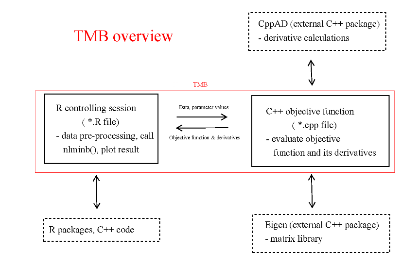
TMB (Template Model Builder) is an R package for fitting statistical latent variable models to data. It is strongly inspired by ADMB. Unlike most other R packages the model is formulated in C++. This provides great flexibility, but requires some familiarity with the C/C++ programming language.
- TMB can calculate first and second order derivatives of the likelihood function by AD, or any objective function written in C++.
- The objective function (and its derivatives) can be called from R. Hence, parameter estimation via e.g.
nlminb()is easy. - The user can specify that the Laplace approximation should be applied to any subset of the function arguments.
- Yields marginal likelihood in latent variable model.
- Standard deviations of any parameter, or derived parameter, obtained by the 'delta method'.
- Pre and post-processing of data done in R.
- TMB is based on state-of-the art software: CppAD, Eigen, ...
A more general introduction including the underlying theory used in TMB can be found in this paper.
Tutorial
A TMB project consists of an R file (*.R) and a C++ file (*.cpp). The R file does pre- and post processing of data in addition to maximizing the log-likelihood contained in *.cpp. See Examples for more details. All R functions are documented within the standard help system in R. This tutorial describes how to write the C++ file, and assumes familiarity with C++ and to some extent with R.
The purpose of the C++ program is to evaluate the objective function, i.e. the negative log-likelihood of the model. The program is compiled and called from R, where it can be fed to a function minimizer like nlminb().
The objective function should be of the following C++ type:
The first line includes the source code for the whole TMB package (and all its dependencies). The objective function is a templated class where <Type> is the data type of both the input values and the return value of the objective function. This allows us to evaluate both the objective function and its derivatives using the same chunk of C++ code (via the AD package CppAD). The technical aspects of this are hidden from the user. There is however one aspect that surprises the new TMB user. When a constant like "1.2" is used in a calculation that affects the return value it must be "cast" to Type:
Obtaining data and parameter values from R
Obviously, we will need to pass both data and parameter values to the objective function. This is done through a set of macros that TMB defines for us.
List of data macros
DATA_ARRAY(),DATA_FACTOR(),DATA_IARRAY(),DATA_IMATRIX(),DATA_INTEGER(),DATA_IVECTOR(),DATA_MATRIX(),DATA_SCALAR(),DATA_SPARSE_MATRIX(),DATA_STRING(),DATA_STRUCT(),DATA_UPDATE(),DATA_VECTOR()
List of parameter macros
PARAMETER(),PARAMETER_ARRAY(),PARAMETER_MATRIX(),PARAMETER_VECTOR()
To see which macros are available start typing DATA_ or PARAMETER_ in the Doxygen search field of your browser (you may need to refresh the browser window between each time you make a new search). A simple example if you want to read a vector of numbers (doubles) is the following
Note that all vectors and matrices in TMB uses a zero-based indexing scheme. It is not necessary to explicitly pass the dimension of x, as it can be retrieved inside the C++ program:
An extended C++ language
TMB extends C++ with functionality that is important for formulating likelihood functions. You have different toolboxes available:
- Standard C++ used for infrastructure like loops etc.
- Vector, matrix and array library (see Matrices and arrays)
- Probability distributions (see Densities and R style distributions)
In addition to the variables defined through the DATA_ or PARAMETER_ macros there can be "local" variables, for which ordinary C++ scoping rules apply. There must also be a variable that holds the return value (neg. log. likelihood).
As in ordinary C++ local variable tmp must be assigned a value before it can enter into a calculation.
Statistical modelling
TMB can handle complex statistical problems with hierarchical structure (latent random variables) and multiple data sources. Latent random variables must be continuous (discrete distributions are not handled). The PARAMETER_ macros are used to pass two types of parameters.
- Parameters: to be estimated by maximum likelihood. These include fixed effects and variance components in the mixed model literature. They will also correspond to hyper parameters with non-informative priors in the Bayesian literature.
- Latent random variables: to be integrated out of the likelihood using a Laplace approximation.
Which of these are chosen is controlled from R, via the random argument to the function MakeADFun. However, on the C++ side it is usually necessary to assign a probability distribution to the parameter.
The purpose of the C++ program is to calculate the (negative) joint density of data and latent random variables. Each datum and individual latent random effect gives a contribution to log likelihood, which may be though of as a "distribution assignment" by users familiar with software in the BUGS family.
The following rules apply:
- Distribution assignments do not need to take place before the latent variable is used in a calculation.
- More complicated distributional assignments are allowed, say u(0)-u(1) ~ N(0,1), but this requires the user to have a deeper understanding of the probabilistic aspects of the model.
- For latent variables only normal distributions should be used (otherwise the Laplace approximation will perform poorly). For response variables all probability distributions (discrete or continuous) are allowed. If a non-gaussian latent is needed the "transformation trick" can be used.
- The namespaces R style distributions and Densities contain many probability distributions, including multivariate normal distributions. For probability distributions not available from these libraries, the user can use raw C++ code:
See Toolbox for more about statistical modelling.
The structure of TMB
This documentation only covers the TMB specific code, not CppAD or Eigen These packages have their own documentation, which may be relevant. In particular, some of the standard functions like sin() and cos() are part of CppAD, and are hence not documented through TMB.
Matrices and arrays
Relationship to R
In R you can apply both matrix multiplication (%*%) and elementwise multiplication (*) to objects of type "matrix", i.e. it is the operator that determines the operation. In TMB we instead have two different types of objects, while the multiplication operator (*) is the same:
matrix: linear algebraarray: elementwise operations; () and [] style indexing.vector: can be used in linear algebra withmatrix, but at the same time admits R style element-wise operations.
See the file matrix_arrays.cpp for examples of use.
Relationship to Eigen
The TMB types matrix and array (in dimension 2) inherits directly from the the Eigen types Matrix and Array. The advanced user of TMB will benefit from familiarity with the Eigen documentation. Note that arrays of dimension 3 or higher are specially implemented in TMB, i.e. are not directly inherited from Eigen.
R style probability distributions
Attempts have been made to make the interface (function name and arguments) as close as possible to that of R.
- The densities (
d...) are provided both in the discrete and continuous case, cumulative distributions (p...) and inverse cumulative distributions (q...) are provided only for continuous distributions. - Scalar and
vectorarguments (in combination) are supported, but notarrayormatrixarguments. - The last argument (of type
int) corresponds to thelogargument in R: 1=logaritm, 0=ordinary scale.true(logaritm) andfalse(ordinary scale) can also be used. - Vector arguments must all be of the same length (no recycling of elements). If vectors of different lengths are used an "out of range" error will occur, which can be picked up by the debugger.
DATA_IVECTOR()andDATA_INTEGER()cannot be used with probability distributions, except possibly for the last (log) argument.- An example:
- To sum over elements in the vector returned use
Multivariate distributions
The namespace
gives access to a variety of multivariate normal distributions:
- Multivariate normal distributions specified via a covariance matrix (structured or unstructured).
- Autoregressive (AR) processes.
- Gaussian Markov random fields (GMRF) defined on regular grids or defined via a (sparse) precision matrix.
- Separable covariance functions, i.e. time-space separability.
These seemingly unrelated concepts are all implemented via the notion of a distribution, which explains why they are placed in the same namespace. You can combine two distributions, and this lets you build up complex multivariate distributions using extremely compact notation. Due to the flexibility of the approach it is more abstract than other parts of TMB, but here it will be explained from scratch. Before looking at the different categories of multivariate distributions we note the following which is of practical importance:
- All members in the
densitynamespace return the negative log density, opposed to the univariate densities in R style distributions.
Multivariate normal distributions
Consider a zero-mean multivariate normal distribution with covariance matrix Sigma (symmetric positive definite), that we want to evaluate at x:
The negative log-normal density is evaluated as follows:
In the last line MVNORM(Sigma) should be interpreted as a multivariate density, which via the last parenthesis (x) is evaluated at x. A less compact way of expressing this is
in which your_dmnorm is a variable that holds the "density".
Note, that the latter way (using the MVNORM_t) is more efficient when you need to evaluate the density more than once, i.e. for different values of x.
Sigma can be parameterized in different ways. Due to the symmetry of Sigma there are at most n(n+1)/2 free parameters (n variances and n(n-1)/2 correlation parameters). If you want to estimate all of these freely (modulo the positive definite constraint) you can use UNSTRUCTURED_CORR() to specify the correlation matrix, and VECSCALE() to specify variances. UNSTRUCTURED_CORR() takes as input a vector a dummy parameters that internally is used to build the correlation matrix via its cholesky factor.
If all elements of dummy_params are estimated we are in effect estimating a full correlation matrix without any constraints on its elements (except for the mandatory positive definiteness). The actual value of the correlation matrix, but not the full covariance matrix, can easily be assessed using the .cov() operator
Autoregressive processes
Consider a stationary univariate Gaussian AR1 process x(t),t=0,...,n-1. The stationary distribution is choosen so that:
- x(t) has mean 0 and variance 1 (for all t).
The multivariate density of the vector x can be evaluated as follows
Due to the assumed stationarity the correlation parameter must satisfy:
- Stationarity constraint: -1 < rho < 1
Note that cor[x(t),x(t-1)] = rho.
The SCALE() function can be used to set the standard deviation.
Now, var[x(t)] = sigma^2. Because all elements of x are scaled by the same constant we use SCALE rather than VECSCALE.
Multivariate AR1 processes
This is the first real illustration of how distributions can be used as building blocks to obtain more complex distributions. Consider the p dimensional AR1 process
The columns in x refer to the different time points. We then evaluate the (negative log) joint density of the time series.
Note the following:
- We have introduced an intermediate variable
your_dmnorm, which holds the p-dim density marginal density of x(t). This is a zero-mean normal density with covariance matrixSigma. - All p univarite time series have the same serial correlation phi.
- The multivariate process x(t) is stationary in the same sense as the univariate AR1 process described above.
Higher order AR processes
There also exists ARk_t of arbitrary autoregressive order.
Gaussian Markov random fields (GMRF)
GMRF may be defined in two ways:
- Via a (sparse) precision matrix Q.
- Via a d-dimensional lattice.
For further details please see GMRF_t. Under 1) a sparse Q corresponding to a Matern covariance function can be obtained via the R_inla namespace.
Separable construction of covariance (precision) matrices
A typical use of separability is to create space-time models with a sparse precision matrix. Details are given in SEPARABLE_t. Here we give a simple example.
Assume that we study a quantity x that changes both in space and time. For simplicity we consider only a one-dimensional space. We discretize space and time using equidistant grids, and assume that the distance between grid points is 1 in both dimensions. We then define an AR1(rho_s) process in space and one in time AR1(rho_t). The separable assumption is that two points x1 and x2, separated in space by a distance ds and in time by a distance dt, have correlation given by
rho_s^ds*rho_t^dt
This is implemented as
Note that the arguments to SEPARABLE() are given in the opposite order to the dimensions of x.
Example collection
- A list of all examples is found on the "Examples" tab on the top of the page.
- Locations of example files:
adcomp/tmb_examplesandadcomp/TMB/inst/examples. - For each example there is both a
.cppand a.Rfile. Take for instance the linear regression example: - C++ template
- Controlling R code
- To run this example use the R command
Example overview
| Example | Description |
|---|---|
| adaptive_integration.cpp | Adaptive integration using 'tiny_ad' |
| ar1_4D.cpp | Separable covariance on 4D lattice with AR1 structure in each direction. |
| compois.cpp | Conway-Maxwell-Poisson distribution |
| fft.cpp | Multivariate normal distribution with circulant covariance |
| hmm.cpp | Inference in a 'double-well' stochastic differential equation using HMM filter. |
| laplace.cpp | Laplace approximation from scratch demonstrated on 'spatial' example. |
| linreg_parallel.cpp | Parallel linear regression. |
| linreg.cpp | Simple linear regression. |
| longlinreg.cpp | Linear regression - 10^6 observations. |
| lr_test.cpp | Illustrate map feature of TMB to perform likelihood ratio tests on a ragged array dataset. |
| matern.cpp | Gaussian process with Matern covariance. |
| mvrw_sparse.cpp | Identical with random walk example. Utilizing sparse block structure so efficient when the number of states is high. |
| mvrw.cpp | Random walk with multivariate correlated increments and measurement noise. |
| nmix.cpp | nmix example from https://groups.nceas.ucsb.edu/non-linear-modeling/projects/nmix |
| orange_big.cpp | Scaled up version of the Orange Tree example (5000 latent random variables) |
| register_atomic_parallel.cpp | Parallel version of 'register_atomic' |
| register_atomic.cpp | Similar to example 'adaptive_integration' using CppAD Romberg integration. REGISTER_ATOMIC is used to reduce tape size. |
| sam.cpp | State space assessment model from Nielsen and Berg 2014, Fisheries Research. |
| sde_linear.cpp | Inference in a linear scalar stochastic differential equation. |
| sdv_multi_compact.cpp | Compact version of sdv_multi |
| sdv_multi.cpp | Multivatiate SV model from Skaug and Yu 2013, Comp. Stat & data Analysis (to appear) |
| socatt.cpp | socatt from ADMB example collection. |
| spatial.cpp | Spatial poisson GLMM on a grid, with exponentially decaying correlation function |
| spde_aniso_speedup.cpp | Speedup "spde_aniso.cpp" by moving normalization out of the template. |
| spde_aniso.cpp | Anisotropic version of "spde.cpp". |
| spde.cpp | Illustration SPDE/INLA approach to spatial modelling via Matern correlation function |
| thetalog.cpp | Theta logistic population model from Pedersen et al 2012, Ecol. Modelling. |
| TMBad/interpol.cpp | Demonstrate 2D interpolation operator |
| TMBad/sam.cpp | State space assessment model from Nielsen and Berg 2014, Fisheries Research. |
| TMBad/solver.cpp | Demonstrate adaptive solver of TMBad |
| TMBad/spa_gauss.cpp | Demonstrate saddlepoint approximation (SPA) |
| TMBad/spatial.cpp | Spatial poisson GLMM on a grid, with exponentially decaying correlation function |
| TMBad/spde_epsilon.cpp | Low-level demonstration of fast epsilon bias correction using 'sparse plus lowrank' hessian |
| TMBad/thetalog.cpp | Theta logistic population model from Pedersen et al 2012, Ecol. Modelling. |
| transform_parallel.cpp | Parallel version of transform |
| transform.cpp | Gamma distributed random effects using copulas. |
| transform2.cpp | Beta distributed random effects using copulas. |
| tweedie.cpp | Estimating parameters in a Tweedie distribution. |
| validation/MVRandomWalkValidation.cpp | Estimate and validate a multivariate random walk model with correlated increments and correlated observations. |
| validation/randomwalkvalidation.cpp | Estimate and validate a random walk model with and without drift |
| validation/rickervalidation.cpp | Estimate and validate a Ricker model based on data simulated from the logistic map |
Compilation and run time errors
The R interface to the debugger (gdb) is documented as part of the R help system, i.e. you can type ?gdbsource in R to get info. The current document only adresses isses that the relate to C++.
Compilation errors
It may be hard to understand the compilation errors for the following reasons
- The Eigen libraries use templated C++ which generate non-intuitive error messages.
Run time errors
Run time errors are broadly speaking of two types:
- Out-of-bounds (you are "walking out of an array")
- Floating point exceptions
You can use the debugger to locate both types of errors, but the procedure is a little bit different in the two cases. The following assumes that you have the GNU debugger gdb installed.
Out-of-bounds error
An example is:
This will cause TMB and R to crash with the following error message:
TMB has received an error from Eigen. The following condition was not met: index >= 0 && index < size() Please check your matrix-vector bounds etc., or run your program through a debugger. Aborted (core dumped)
So, you must restart R and give the commands
#5 objective_function<double>::operator() (this=<optimized out>="">) at nan_error_ex.cpp:11
and you can see that the debugger points to line number 11 in the .cpp file. gdbsource() is an R function that is part of TMB.
Floating point exception
If you on the other hand perform an illegal mathematical operation, such as
R will not crash, but the objective function will return a NaN value. However, you will not know in which part of your C++ code the error occured. By including the fenv.h library (part of many C++ compilers, but can otherwise be downloaded from http://www.scs.stanford.edu/histar/src/uinc/fenv.h)
nan_error_ex.cpp:
a floating point exception will be turned into an actual error that can be picked up by the debugger. There are only two extra lines that need to be included ("//Extra line needed" in the above example).
When we try to run this program in the usual way, the program crashes:
Floating point exception (core dumped) tmp3>
At this stage you should run the debugger to find out that the floating point exception occurs at line number 14:
#1 0x00007ffff0e7eb09 in objective_function<double>::operator() (this=<optimized out>="">) at nan_error_ex.cpp:14
This enabling of floating point errors applies to R as well as the TMB program. For more elaborate R-scripts it may therefore happen that a NaN occurs in the R-script before the floating point exception in the TMB program (i.e. the problem of interest) happens. To circumvent this problem one can run without NaN debugging enabled and save the parameter vector that gave the floating point exception (e.g. badpar <- obj$env$last.par after the NaN evaluation), then enable NaN debugging, re-compile, and evaluate obj$env$f( badpar, type="double").
Missing casts for vectorized functions
TMB vectorized functions cannot be called directly with expressions, for example the following will fail to compile:
error: could not convert ‘atomic::D_lgamma(const CppAD::vector<Type>&) ... from ‘double’ to ‘Eigen::CwiseBinaryOp<Eigen::internal::scalar_sum_op<double, double>, ... >’
Eigen lazy-evaluates expressions, and the templating of lgamma means we expect to return a "x + y"-typed object, which it obviously can't do.
To work around this, cast the input:
Toolbox
First read the Statistical Modelling section of Tutorial.
Non-normal latent variables (random effects)
The underlying latent random variables in TMB must be Gaussian for the Laplace approximation to be accurate. To obtain other distributions, say a gamma distribution, the "transformation trick" can be used. We start out with normally distributed variables u and transform these into new variables w via the pnorm and qgamma functions as follows:
w now has a gamma distribution.
Discrete latent variables
The Laplace approximation can not be applied to discrete latent variables that occur in mixture models and HMMs (Hidden Markov models). However, such likelihoods have analytic expressions, and may be coded up in TMB. TMB would still calculate the exact gradient of the HMM likelihood.
Mixture models
Although mixture models are a special case of discrete latent variable models, they do deserve special attention. Consider the case that we want a mixture of two zero-mean normal distributions (with different standard deviations). This can be implemented as:
Time series
Autoregressive (AR) processes may be implemented using the compact notation of section Densities. The resulting AR process may be applied both in the observational part and in the distribution of a latent variable.
Nonlinear time must be implemented from scratch, as in the example thetalog.cpp
Spatial models
TMB has strong support for spatial model and space-time models via the GMRF() and SEPARABLE() functions, and the notion of a distribution. The reader is referred to section Densities for details and examples.
C++ tutorial
I know R but not C++
Summary of how syntax differs between R and C++:
It is important to note the following difference compared to R:
Vectors, matrices and arrays are not zero-initialized in C++.
A zero initialized object is created using Eigens setZero():
I know C++
TMB specific C++ include:
- You should not use
if(x)statements wherexis aPARAMETER, or is derived from a variable of typePARAMETER. (It is OK to useifonDATAtypes, however.) TMB will remove theif(x)statement, so the code will produce unexpected results.